Category: Interesting External Papers

Contingent Capital

Contingent Capital: Reverse Convertible Debentures

Mark J. Flannery Bank of America Eminent Scholar Chair of Finance at the University of Florida proposed Reverse Convertible Debentures in 2002 in his paper No Pain, No Gain? Effecting Market Discipline via “Reverse Convertible Debentures”:

The deadweight costs of financial distress limit many firms’ incentive to include a lot of (taxadvantaged) debt in their capital structures. It is therefore puzzling that firms do not make advance arrangements to re-capitalize themselves if large losses occur. Financial distress may be particularly important for large banking firms, which national supervisors are reluctant to let fail. The supervisors’ inclination to support large financial firms when they become troubled mitigates the ex ante incentives of market investors to discipline these firms. This paper proposes a new financial instrument that forestalls financial distress without distorting bank shareholders’ risk-taking incentives. “Reverse convertible debentures” (RCD) would automatically convert to common equity if a bank’s market capital ratio falls below some stated value. RCD provide a transparent mechanism for un-levering a firm if the need arises. Unlike conventional convertible bonds, RCD convert at the stock’s current market price, which forces shareholders to bear the full cost of their risk-taking decisions. Surprisingly, RCD investors are exposed to very limited credit risk under plausible conditions.

Of interest is the example of some Manny-Hanny bonds:

The case of Manufacturers Hanover (MH) in 1990 illustrates the problem. The bank had issued $85 million dollars worth of “mandatory preferred stock,” which was scheduled to convert to common shares in 1993. An earlier conversion would be triggered if MH’s share price closed below $16 for 12 out of 15 consecutive trading days (Hilder [1990]). Such forced conversion appeared possible in December 1990. In a letter to the Federal Reserve Bank of New York concerning the bank’s capital situation, MH’s CFO (Peter J. Tobin) expresses the bank’s extreme reluctance to permit conversion, or to issue new equity at current prices. At yearend 1990, MH’s book ratio of equity capital to total (on-book) assets was 5.57%, while its market equity ratio was 2.53%. The bank was also adamant in announcing that it would not omit its quarterly dividend. Despite the low market capital ratio, the Fed appeared unable to force MH to issue new equity. Chemical Bank acquired Manufacturers Hanover at the end of 1991.

When Manufacturers’ Hanover confronted a possible conversion of preferred stock in late 1990 (see footnote 6), they considered redeeming the issue using cash on hand. Such a “plan” only works if a supervisor will accept it. Under a market value trigger, such redemption would have to be financed by issuing equity; otherwise, the redemption would further lower the capital ratio. Another important feature of the MH convertible preferred issue was that the entire issue converted if common share prices were even $.01 too low over the specified time interval.

Flannery proposes the following design parameters for RCD:

RCD would have the following broad design features:

  • 1. They automatically convert into common equity if the issuer’s capital ratio falls below a pre-specified value.
  • 2. Unless converted into shares, RCD receive tax-deductible interest payments and are subordinated to all other debt obligations.
  • 3. The critical capital ratio is measured in terms of outstanding equity’s market value. (See Section III.)
  • 4. The conversion price is the current share price. Unlike traditional convertible bonds, one dollar of debentures (in current market value) would generally convert into one dollar’s worth of common stock.
  • 5. RCD incorporate no options for either investors or shareholders: conversion occurs automatically when the trigger is tripped.
  • 6. When debentures convert, the firm must promptly sell new RCD to replace the converted ones.

An example of RCD conversion is provided:

The bank in Figure 1 starts out at t = 0 with a minimally acceptable 8% capital ratio, backed by RCD equal to an additional 5% of total assets. With ten shares (“N”) outstanding, the initial share price (“PS”) is $0.80. By t = ½, the bank’s asset value has fallen to $97, leaving equity at $5.00 and the share price at $0.50. The bank is now under-capitalized ($5/$97 = 5.15% < 8%). Required capital is $7.76 (= 8% of $97). The balance sheet for t = 1 shows that $2.76 of RCD converted into equity to restore capital to 8% of assets. Given that PS = $0.50 at t = ½, RCD investors receive 5.52 shares in return for their $2.76 of bond claims. These investors lose no principal value when their debentures convert: they can sell their converted shares at $0.50 each and use the proceeds to re-purchase $2.76 worth of bonds. The initial shareholders lose the option to continue operating with low equity, because they must share the firm’s future cash flows with converted bondholders.

The critical part of this structure is that the triggering capital ratio values outstanding equity at market prices, rather than book. Additionally, not all – not necessarily even all of one issue – gets converted. Flannery suggests that issues be converted in the order of their issuance; first-in-first-out.

A substantial part of the paper consists of a defense of this market value feature, which I shall not reproduce here.

Flannery repeatedly touts a feature of the plan that I consider a bug:

Triggered by a frequently-evaluated ratio of equity’s market value to assets, RCD could be nearly riskless to the initial investors, while transmitting the full effect of poor investment outcomes to the shareholders who control the firm.

I don’t like the feature. I believe that a fixed-price conversion with a fixed-price trigger will aid in the analysis of this type of issue and make it easier for banks to sell equity above the trigger point – which is desirable! It is much better if the troubled bank can sell new equity to the public at a given price than to have the RCDs convert – Flannery worries about a requirement that the banks replace converted RCDs in short order, which is avoided if the trigger is avoided. If new equity prospects are not aware of their possible dilution if bad times become even worse, they will be less eager to buy.

Additionally, I am not enamoured of the use of regulatory asset weightings as a component of the trigger point. The last two years have made it very clear that there is a very wide range of values that may be assigned to illiquid assets; honest people can legitimately disagree, sometimes by amounts that are very material.

Market trust in the quality of the banks’ mark-to-market of its assets will be reflected, at least to some degree, by the Price/Book ratio. So let’s re-work Flannery’s Table 1 for two banks; both with the same initial capitalization; both of which mark down their assets by the same amount; but one of which maintains its Price/Book ratio (investors trust bank management) while the other’s P/B ratio declines (investors don’t trust bank management, or for some other reason believe that the end of the write-downs is yet to come).

Note that Flannery’s specification for the Market Ratio:

The market value equity ratio is the market value of common stock divided by the sum of (the book value of total liabilities plus the market value of common stock).

Two banks: t=0
Trusty Bank
Assets Liabilities
100 87 Deposits
5 RCD
8 Equity
N = 10, Book = $0.80, Price = $1.20;
Market Ratio = 12/(87+5+12) = 11.5%
Sleazy Bank
Assets Liabilities
100 87 Deposits
5 RCD
8 Equity
N = 10, Book = $0.80, Price = $1.20;
Market Ratio = 12/(87+5+12) = 11.5%

This is basically the same as Flannery’s example; however, he uses a constant P/B ratio of 1.0 to derive a Market Ratio of 8%. In addition, I will assume that the regulatory requirement for the Market Ratio is 10% – the two banks started with a cushion.

Disaster strikes at time t=0.5, when asset values decline by 3%. Trusty Bank’s P/B remains constant at 1.5, but Sleazy Bank’s P/B declines to 0.8.

Two banks: t=0.5
Trusty Bank
Assets Liabilities
97 87 Deposits
5 RCD
5 Equity
N = 10, Book = $0.50, Price = $0.75;
Market Ratio = 7.50 / (87+5+7.5) = 7.54%
Sleazy Bank
Assets Liabilities
97 87 Deposits
5 RCD
5 Equity
N = 10, Book = $0.50, Price = $0.40;
Market Ratio = 4.00 / (87+5+4) = 4.17%

In order to get its Market Ratio back up to the 10% regulatory minimum that is assumed, Trusty Bank needs to solve the equation:

[7.5+x] / [87 + (5-x) + (7.5 + x)] = 0.10

where x is the Market Value of the new equity and is found to be equal to 2.45. With a stock price of 0.75, this is equal to 3.27 shares

Sleazy Bank solves the equation:

[4.0+x] / (87 + (5-x) + (4.0 +x)) = 0.10

and finds that x is 5.60. With a stock price of 0.40, this is equal to 14.00 shares.

Two banks: t=1.0
Trusty Bank
Assets Liabilities
97 87 Deposits
2.55 RCD
7.45 Equity
N = 13.27, Book = $0.56, Price = $0.75;
Market Ratio = (13.27*0.75)/(87+2.55+(13.27*0.75)) = 10%
Sleazy Bank
Assets Liabilities
97 87 Deposits
-0.60 RCD
10.60 Equity
N = 24.00, Book = $0.44, Price = $0.40;
Market Ratio = (24*0.4)/(87-0.6+(24*0.4)) = 10%

Sleazy Bank doesn’t have the capital on hand – as shown by the negative value of balance sheet RCD at t=1 – so it goes bust instead. In effect, there has been a bank run instigated not by depositors but by shareholders.

Note that in the calculations I have assumed that the price of the common does not change as a result of the dilution; this alters the P/B ratio. Trusty Bank’s P/B moves from 1.50 to 1.34; Sleazy Bank’s P/B (ignoring the effect of the negative value of the RCDs) moves from 0.8 to 0.91. Whether or not the assumption of constant market price is valid in the face of the dilution is a topic that can be discussed at great length.

I will note that the Price/Book ratio of Japanese banks in early 2008 was 0.32:1 and Citigroup’s P/B ratio is currently 0.67:1.

While Dr. Flannery’s idea has its attractions, I am very hesitant about the idea of mixing book and market values. From a theoretical viewpoint, capital is intended to be permanent, which implies that once the bank has its hands on the money, it doesn’t really care all that much about the price its capital trades at in the market.

Using a fixed conversion price, with a fixed market price trigger keeps the separation of book accounting from market pricing in place, which offers greater predictability to banks, investors and potential investors in times of trouble.

Update 2009-11-1: Arithmetical error corrected in table.

It should also be noted that the use of market value of equity in calculating regulatory ratios makes the proposal as it stands extremely procyclical.
Interesting External Papers

Stop-Loss Orders

Stop-Loss Orders have always seemed completely insane to me. They completely ignore fundamentals; they are set according to price only.

If you’re willing to sell something at $20, why wouldn’t you sell it at $21 when you have the chance? The deliberate introduction of negative convexity into a portfolio – without getting paid for it! – is something that has bothered me even before I could express the idea in terms of convexity.

I was asked a question regarding Stop-Loss orders recently, which I answered as politely as I could; but it would be helpful to have some academic references to buttress my biases … or, who knows, maybe even refute them, although that would be the complete antithesis of how I have managed money throughout my career.

So … I’m starting this post to keep my notes in. Carry on!

Positive Feedback Investment Strategies and Destabilizing Rational Speculation, J. Bradford De Long, Andrei Shleifer, Lawrence H. Summers and Robert J. Waldmann. Yep, that’s THE Larry Summers. Anyway, the argument here is that there will be a certain proportion of “positive feedback” traders in the market, no matter what – they might even be margin traders, getting margin calls in a down market. Therefore, it becomes rational for informed traders to overreact to actual news, because they know that uninformed traders will overreact even more while the informed traders liquidate. While interesting, the authors are more interested in demonstrating the variability of the market and determining “critical points” – where a decline becomes a discontinuous crash – rather than looking at empirical evidence of stop-loss profit-and-loss.

Market Liquidity, Hedging, and Crashes by Gerard Gennotte and Hane Leland has much the same theme. There’s a nice line in the conclusion: “Traditional models which do not recognize that many investors are poorly informed will grossly overestimate the liquidity of stock markets” …. I’ll have to think about how that might tie in with the Credit Cruch!

Contingent Capital

OSFI Joins Contingent Capital Bandwagon

The Office of the Superintendent of Financial Institutions (OSFI) has released a speech by Julie Dickson to the C.D. Howe Institute titled Considerations along the Path to Financial Regulatory Reform.

The most important part was the section on contingent capital:

Explore the use of contingent capital. This refers to sizeable levels of lower quality capital that could convert into high quality capital at pre-specified points, and clearly before an institution could receive government support. Such conversions could make use of triggers in the terms of a bank’s lower quality capital, while the bank remains a going-concern. This would add market discipline for even the largest banks during good times (as common shareholders could be significantly diluted in an adverse scenario), while stabilizing the situation by recapitalizing such banks if they fall on hard times. Boards and management of these recapitalized banks could be replaced. Issues to be studied to make such a proposal operational include grandfathering of existing lower quality securities, and/or transitioning towards new features in lower quality securities, considering capital markets implications of changing the terms of lower quality capital and the selection of triggers, and determining the amounts and market for such instruments.

Contingent capital was first proposed in such a form – as far as I know! – in HM Treasury’s response to the Turner Report.

Under the heading Making Failure a Viable Option, she advocates:

More control of counterparty risk via capital rules and limits, so that imposing losses on major institutions who are debt holders in a failed financial institution does not prove fatal.

It is possible that this might be an attack on the utterly ridiculous Basel II risk weighting of bank paper according to the credit rating of the bank’s supervisor; that is, paper issued by a US bank is risk-weighted according to the credit rating of the US, which is perhaps the most difficult thing to understand about the Basel Rules. If the regulators are serious about reducing systemic risk, then paper issued by other financial institutions should attract a higher risk weighting than that of a credit-equivalent non-financial firm, not less.

I have often remarked on the Bank of Canada’s attempts to expand its bureaucratic turf throughout the crisis; two can play at that game!

one could try to experiment and adjust capital requirements up or down based on macro indicators. But, the challenge will be how to make a regime which ties macro indicators to capital effective. Indeed, in upturns in the domestic market where capital targets are increased due to macro factors, companies would have the option to obtain loans from banks in countries with less robust economic conditions, as banks in that country will have lower requirements. Thus, an increase in capital in the domestic market might not have the desired impact of slowing things down.

Alternatively, because many countries have well developed financial sectors, borrowers can go beyond the regulated financial sector to find money, as regulated financial institutions are not the only game in town.

Umm … hello? The objective of varying credit requirements is to strengthen the banks should there be a possible downturn; the Greenspan thesis is that it is extremely difficult to tell if you’re in a bubble while you’re in the middle of it (and therefore, you do more damage by prevention than is done by cure) has attracted academic support (as well as being simple common sense; if a bubble was obvious, it wouldn’t exist).

Most authorities agree that Central Banks have the responsibility for “slowing things down” via monetary policy; OSFI should stick to its knitting and concentrate on assuring the relative health of the regulated financial sector it regulates.

Of particular interest is her disagreement with one element of Treasury’s wish-list:

Yes, regulators should try to assess systemic risk. But no, we should not try to define systemically important financial institutions.

The IMF work on identifying systemic institutions rightly points out that what is systemic in one situation may not be in another, and that there is considerable judgement involved.

Ms. Dickson also made several remarks about market discipline, which should not be taken seriously.

Update: I’ve been trying to find the “IMF work” referred to in the last quoted paragraph; so far, my best guess is Chapter 3 of the April ’09 Global Financial Stability Report:

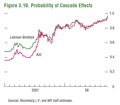
Cascade effects. Another use of the joint probability distribution is the probability of cascade effects, which examines the likelihood that one or more FIs in the system become distressed given that a specific FI becomes distressed. It is a useful indicator to quantify the systemic importance of a specific FI, since it provides a direct measure of its effect on the system as a whole. As an example, the probability of cascade effects is estimated given that Lehman or AIG became distressed. These probabilities reached 97 percent and 95, respectively, on September 12, 2008, signaling a possible “domino” effect in the days after Lehman’s collapse (Figure 3.10). Note that the probability of cascade effects for both institutions had already increased by August 2007, well before Lehman collapsed.

The IMF Country Report No. 09/229 – United States: Selected Issues points out:

It remains to be seen how the Federal Reserve, in consultation with the Treasury, will draw up rules to guide the identification of systemic firms to be brought under its purview, and how the FSOC will ensure that remaining intermediaries are monitored from a broader financial stability perspective. Although the criteria for Tier 1 FHC status appropriately include leverage and interconnectedness as well as size, identifying systemic institutions ex ante will remain a difficult task (cf., AIG).

I have sent an inquiry to OSFI asking for a specific reference.

Update, 2009-11-9: OSFI’s bureaucrats have not seen fit to respond to my query, but the Bank for International Settlements has just published the Report to G20 Finance Ministers and Governors: Guidance to Assess the Systemic Importance of Financial Institutions, Markets and Instruments: Initial Considerations which includes the paragraph:

The assessment is likely to be time-varying depending on the economic environment. Systemic importance will depend significantly on the specifics of the economic environment at the time of assessment. Structural trends and the cyclical factors will influence the outcome of the assessment. For instance, under weak economic conditions there is a higher probability that losses will be correlated and failures in even relatively unimportant elements of the financial sector could become triggers for more general losses of confidence. A loss of confidence is often associated with uncertainty of asset values, and can manifest in a contagious “run” on short-run liabilities of financial institutions, or more generally, in a loss of funding for key components of the system. The dependence of the assessment on the specific economic and financial environment has implications about the frequency with which such assessments should take place, with the need for more frequent assessments to take account of new information when financial systems are under stress or where material changes in the environment or the business and risk profile of the individual component have taken place.

It is regrettable that OSFI does not have a sufficiently scholarly approach to its work to provide references in the published version of Julie Dickson’s speeches – or that she would not insist on such an approach. It is equally regrettable that OSFI is unable to answer a simple question regarding such a reference within a day or so.

Interesting External Papers

Subprime mortgages: Myths and reality

The paper Understanding the Subprime Mortgage Crisis by Yuliya S. Demyanyk and Otto Van Hemert has been previously discussed on PrefBlog, but it’s about to be published on a formal basis (forthcoming in the Review of Financial Studies) and the authors are beating the drums for it on VoxEU.

In the essay Subprime mortgages: Myths and reality, they highlight the following sources of confusion about the Credit Crunch:

  • Myth: Subprime mortgages went only to borrowers with impaired credit
  • Myth: Subprime mortgages promoted homeownership
  • Myth: Declines in mortgage underwriting standards triggered the subprime crisis
  • Myth: Subprime mortgages failed because people used homes as ATMs
  • Myth: Subprime mortgages failed because of mortgage rate resets
  • Myth: Subprime borrowers with hybrid mortgages were offered (low) “teaser rates”

Their conclusion is in line with what I’ve been saying for some time:

Many of the myths presented here single out some characteristic of subprime loans, subprime borrowers, or the economic circumstances in which those loans were made as the cause of the crisis. All of these factors are certainly important for borrowers with subprime mortgages in terms of their ability to keep their homes and make regular mortgage payments. But no single factor is responsible for the subprime failure.

In hindsight, the subprime crisis fits neatly into the classic lending boom and bust story – subprime mortgage lending experienced a remarkable boom, during which the market expanded almost sevenfold over six years. In each of these years between 2001 and 2007, the quality of mortgages was deteriorating, their overall riskiness was increasing, and the pricing of this riskiness was decreasing (see Demyanyk and Van Hemert 2008). For years, rising house prices concealed the subprime mortgage market’s underlying weaknesses and unsustainability. When this veil was finally pulled away by a nationwide contraction in prices, the true quality of the loans was revealed in a vast wave of delinquencies and foreclosures that continues to destabilise the US housing market even today.

Subprime is just another boom and bust story; just another example of the manner in which easy money will find an outlet. Usually, of course, easy money will express itself in terms of inflation; since there was not much inflation in the period 2001-07, the Fed missed the underlying problem. This isn’t just my thesis: it has been suggested by Ken Taylor of Taylor Rule fame and researchers from the Kansas City Fed.

Unfortunately, the politicians have taken over public discussion of the issue and find it much more convenient to blame bankers and their compensation; when, in fact, these guys are in the same position as those poor suckers who get caught by customs with a suitcase-full of heroin. Yes, they did wrong; but it is more important to find out who filled the suitcase.

Interesting External Papers

BoC Research: Monetary Policy and FX-Driven Inflation

The Bank of Canada has released Working Paper 2009-29 by Stephen Murchison titled Exchange Rate Pass-Through and Monetary Policy: How Strong is the Link?:

Several authors have presented reduced-form evidence suggesting that the degree of exchange rate pass-through to the consumer price index has declined in Canada since the early 1980s and is currently close to zero. Taylor (2000) suggests that this phenomenon, which has been observed for several other countries, may be due to a change in the behaviour of inflation. Specifically, moving from a high to a low-inflation environment has reduced the expected persistence of cost changes and, by consequence, the degree of pass-through to prices. This paper extends his argument, suggesting that this change in persistence is due to a change in the parameters of the central bank’s policy rule. Evidence is presented for Canada indicating that policy has responded more aggressively to inflation deviations over the low pass-through period relative to the high pass-through period. We test the quantitative importance of this change in policy for exchange rate pass-through by varying the parameters of a simple monetary policy rule embedded in an open economy, dynamic stochastic general equilibrium model. Results suggest that increases in the aggressiveness of policy consistent with that observed for Canada are sufficient to effectively eliminate measured pass-through. However, this conclusion depends critically on the inclusion of price-mark-up shocks in the model. When these are excluded, a more modest decline to pass-through is predicted.

He uses a model incorporating a Taylor Rule for policy rates and finds:

Overall, we find that for reasonable changes to the policy rule, large changes in estimated pass-through can be generated. Specifically, parameter values of between 1.6 and 2.1 on the deviation of in‡ation from target (in a Taylor rule) are sufficient cient to drive estimated pass-through to zero.

The author concludes, in part:

In particular, small changes in policy can have a profound effect on the correlation between prices and the exchange rate in the presence of mark-up shocks and this is largely responsible for the result. When mark-up shocks are excluded from the model or when pass-through is defined in terms of the response of prices to a deterministic exchange-rate shock, we conclude that more aggressive monetary policy in Canada has likely reduced pass-through by about 50 per cent relative to its level prior to 1984.

Interesting External Papers

The US Dollar Shortage & Policy Response

The Bank for International Settlements has released a paper by Patrick McGuire and Goetz von Peter titled The US dollar shortage in global banking and the international policy response:

Among the policy responses to the global financial crisis, the international provision of US dollars via central bank swap lines stands out. This paper studies the build-up of stresses on banks’ balance sheets that led to this coordinated policy response. Using the BIS international banking statistics, we reconstruct the worldwide consolidated balance sheets of the major national banking systems. This allows us to investigate the structure of banks’ global operations across their offices in various countries, shedding light on how their international asset positions are funded across currencies and counterparties. The analysis first highlights why a country’s “national balance sheet”, a residency-based measure, can be a misleading guide to where the vulnerabilities faced by that country’s national banking system (or residents) lie. It then focuses on banking systems’ consolidated balance sheets, and shows how the growth (since 2000) in European and Japanese banks’ US dollar assets produced structural US dollar funding requirements, setting the stage for the dollar shortage when interbank and swap markets became impaired.

The swap lines arranged by the Fed (reported on PrefBlog on 2008-9-29) have been a topic of great fascination for me as the details have been explained; most recently in the BIS Quarterly Review of March 2009.

We find that, since 2000, the Japanese and the major European banking systems took on increasingly large net (assets minus liabilities) on-balance sheet positions in foreign currencies, particularly in US dollars. While the associated currency exposures were presumably hedged off-balance sheet, the build-up of net foreign currency positions exposed these banks to foreign currency funding risk, or the risk that their funding positions (FX swaps) could not be rolled over.

This yields a lower-bound estimate of banks’ US dollar funding gap – the amount of short-term US dollar funding banks require – measured here as the net amount of US dollars channelled to non-banks. By this estimate, European banks’ need for short-term US dollar funding was substantial at the onset of the crisis, at least $1.0–1.2 trillion by mid-2007.

Events during the crisis led to severe disruptions in banks’ sources of short-term funding. Interbank markets seized up, and dislocations in FX swap markets made it even more expensive to obtain US dollars via swaps. Banks’ funding pressures were compounded by instability in non-bank sources of funds as well, notably dollar money market funds and dollar-holding central banks. The market stress meant that the effective maturity of banks’ US dollar funding shortened just as that of their US dollar assets lengthened, since many assets became difficult to sell in illiquid markets.

Consider a bank that seeks to diversify internationally, or expand its presence in a specific market abroad. This bank will have to finance a particular portfolio of loans and securities, some of which are denominated in foreign currencies (eg a German bank’s investment in US dollar-denominated structured finance products). The bank can finance these foreign currency positions in several ways:

  • 1. The bank can borrow domestic currency, and convert it in a straight FX spot transaction to purchase the foreign asset in that currency.
  • 2. It can also use FX swaps to convert its domestic currency liabilities into foreign currency and purchase the foreign assets.
  • 3. Alternatively, the bank can borrow foreign currency, either from the interbank market, from non-bank market participants or from central banks.

The first option produces no subsequent foreign currency needs, but exposes the bank to currency risk, as the on-balance sheet mismatch between foreign currency assets and domestic currency liabilities remains unhedged. Our working assumption is that banks employ FX swaps and forwards to hedge any on-balance sheet currency mismatch.

So in other words, it’s just another wrinkle on the same old story: borrow short + lend long = funding risk. But it’s a good wrinkle!

Why is funding risk in foreign currencies of special interest? Banks also face the risks inherent in transforming maturities in their domestic currency market, of course. However, in a purelydomestic banking context, the central bank can act as lender of last resort and provide sufficient liquidity to eliminate a domestic funding shortage; doing so is both time-honoured practice (Bagehot (1873), Goodhart (1995)) as well as optimal policy (Allen and Gale (1998), Diamond and Rajan (2006)). By contrast, central banks cannot create foreign currencies; their ability to meet banks’ demand for foreign currencies is constrained by the exchange rate regime or limited to available FX reserves (Chang and Velasco (2000, 2001), Obstfeld et al (2009)). Banks’ foreign currency requirements may therefore have to be met from international sources (Fischer (1999), Mishkin (1999)).

It gets better:

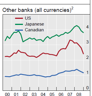
The origins of the US dollar shortage during the crisis are linked to the expansion since 2000 in banks’ international balance sheets. The outstanding stock of banks’ foreign claims grew from $10 trillion at the beginning of 2000 to $34 trillion by end-2007, a significant expansion even when scaled by global economic activity (Figure 1, left panel).For example, Swiss banks’ foreign claims jumped from roughly five times Swiss nominal GDP in 2000 to more than seven times in mid-2007 (Table 1). Dutch, French, German and UK banks’ foreign claims expanded considerably as well. In contrast, Canadian, Japanese and US banks’ foreign claims grew in absolute terms over the same period, but did not significantly outpace the growth in domestic or world GDP (Figure 1, right Panel).


This is the Right Panel.
Click for the whole thing

The lack of foreign funding pressure might be a more precise indication of why Canadian banks were resilient during the crisis.

Then Bad Things happened:

European banks’ funding difficulties were compounded by instability in the non-bank sources of funds as well. Money market funds, facing large redemptions following the failure of Lehman Brothers, withdrew from bank-issued paper, threatening a wholesale run on banks (Baba et al (2009)). Less abruptly, a portion of the US dollar foreign exchange reserves that central banks had placed with commercial banks was withdrawn during the course of the crisis. In particular, some monetary authorities in emerging markets reportedly withdrew placements in support of their own banking systems in need of US dollars.

Market conditions during the crisis have made it difficult for banks to respond to these funding pressures by reducing their US dollar assets. While European banks held a sizeable share of their net US dollar investments as (liquid) US government securities (Figure 5, bottom right panel), other claims on non-bank entities – such as structured finance products – have been harder to sell into illiquid markets without realising large losses. Other factors also hampered deleveraging of US dollar assets: banks brought off-balance sheet vehicles back onto their balance sheets and prearranged credit commitments were drawn.

But … Fed to the rescue!

On 13 October 2008, the swap lines between the Federal Reserve and the Bank of England, the ECB and the Swiss National Bank became unlimited to accommodate any quantity of US dollar funding demanded. The swap lines provided these central banks with ammunition beyond their existing foreign exchange reserves (Obstfeld et al (2009)), which in mid-2007 amounted to $294 billion for the euro area, Switzerland and the United Kingdom combined, an order of magnitude smaller than our lower-bound estimate of the US dollar funding gap.

In providing US dollars on a global scale, the Federal Reserve effectively engaged in international lending of last resort. The swap network can be understood as a mechanism by which the Federal Reserve extends loans, collateralised by foreign currencies, to other central banks, which in turn make these funds available through US dollar auctions in their respective jurisdictions.33 This made US dollar liquidity accessible to commercial banks around the world, including those that have no US subsidiaries or insufficient eligible collateral to borrow directly from the Federal Reserve System.

The authors conclude, in part:

What pushed the system to the brink was not cross-currency funding per se, but rather too many large banks employing funding strategies in the same direction, the funding equivalent of a “crowded trade”. Only when examined at the aggregate level can such vulnerabilities be identified. By quantifying the US dollar overhang on non-US banks’ global balance sheets, this paper contributes to a better understanding of why the extraordinary international policy response was necessary.

and why it took the form of a global network of central bank swap lines.

Interesting External Papers

Stock / Bond Correlation and Financial Stress

Just a quick note here … the Kansas City Fed published a paper by Craig S. Hakkio and William R. Keeton titled Financial Stress: What Is It, How Can It Be Measured and Why Does It Matter?.

One of the coefficients is the stock/bond correlation.

Correlation between returns on stocks and Treasury bonds. In normal times, the returns on stocks and government bonds are either unrelated or move together in response to changes in the risk-free discount rate. In times of financial stress, however, investors may view stocks as much riskier than government bonds. If so, they will shift out of stocks into bonds, causing the returns on the two assets to move in opposite directions. A number of studies, some for the United States and some for other countries, confirm that the correlation between stock returns and government bond returns tends to turn negative during financial crises (Andersson and others; Baur and Lucey; Connolly and others; Gonzalo and Olmo). Thus, the stock-bond correlation provides an additional measure of the flight to quality during periods of financial stress. This correlation is computed over rolling three month periods using the S&P 500 and a 2-year Treasury bond index. Also, the negative value of the correlation is used in the KCFSI, so that increases in the measure correspond to increases in financial stress.

The authors are somewhat critical of the Bank of Canada Stress Index:

It includes some variables, such as exchange rate volatility, that are more important for a small open economy like Canada’s than for the United States. It includes the slope of the yield curve, which likely reveals more about the stance of monetary policy than financial stress. And it fails to include any measures of investor uncertainty about bank stock prices.

There appears to be some predictive value in the index:

As shown in the accompanying box, high values of the KCFSI have tended to either coincide with or precede tighter credit standards over the last 20 years. This evidence suggests that changes in credit standards provide an additional channel through which financial stress may affect economic activity.

Regretably, the authors do not dicuss whether these changes in credit standards can be better predicted by other methodologies. I have the same problem with their analysis of the predictive power of the KCFSI on the value of the Chicago Fed National Activity Index.

The authors suggest that the KCFSI could be used to help time the Fed’s exit strategy for the current crisis, but are, frankly, rather unconvincing.

Anyway, the index is down again for September, after a huge decline from the October 2008 peak, but still above July 2007.

Interesting External Papers

Boston Fed Releases TIPS Discussion Paper

The Federal Reserve Bank of Boston has released a Public Policy Discussion Paper by Michelle L. Barnes, Zvi Bodie, Robert K. Triest, and J. Christina Wang titled A TIPS Scorecard: Are TIPS Accomplishing What They Were Supposed to Accomplish? Can They Be Improved?:

In September 1997, the U.S. Treasury developed the TIPS market in order to achieve three important policy objectives: (1) to provide consumers with a class of assets that allows for hedging against real interest rate risk, (2) to provide holders of nominal contracts a means of hedging against inflation risk, and (3) to provide everyone with a reliable indicator of the term structure of expected inflation. This paper evaluates progress toward the achievement of these objectives and analyzes prospective ways to better meet these objectives in the future, by, for example, extending the maturity of TIPS and/or the use of inflation indexes suited to particular geographic regions or demographics. We conclude by arguing that while it is tempting to consider completing markets by introducing more TIPS‐like securities indexed to inflation rates more tailored to particular demographics, our analysis suggests that TIPS indexed to CPI do, in fact, facilitate good synthetic hedges against unexpected changes in inflation for many different investors, since the various inflation measures are very highly correlated. We do, however, argue for extending the maturity of TIPS.

The authors do not assess the cost/benefit profile of TIPS issuance to Treasury as was discussed by, for instance, FRBNY CEO William Dudley earlier this year. The organization of the paper is:

Section II describes TIPS in more detail, emphasizing how they are designed to act as protection against changes in inflation, the tax implications for investors, the demographics of holders of TIPS, and other considerations relating to whether or not TIPS should yield measures of break‐even inflation rates comparable with survey measures of consumers’ inflation expectations or future realized rates of inflation. Section III outlines and evaluates the criticisms of the CPI and speaks to whether its potential mismeasurement is relevant to the efficacy of TIPS as a hedging instrument to guarantee the real return. It also discusses whether the CPI is a good measure for everyone, and whether there might be more appropriate measures for certain heterogeneous groups, along with the costs and benefits of issuing such securities. Section IV demonstrates the efficacy of TIPS as a hedge against various ex ante and ex post inflation measures, as well as the efficacy of TIPS as a short‐term versus a long‐term hedge. The final section concludes with implications for the design of the TIPS market.

There’s rather a neat section on inflation forecasting:

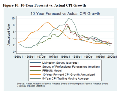
All of the expected inflation measures are largely backward‐looking, moving with recent actual rates of inflation and often deviating substantially from the actual inflation rates that would be experienced over the subsequent 10 years. This is not surprising: although there was concern about the effect of an overheated economy on short‐term inflation rates during the 1960s, it would have been essentially impossible at that time to forecast the oil shocks of the 1970s, or the response of the fiscal and monetary authorities to those shocks. Moreover, the notion of a vertical long‐run Phillips curve was still controversial among economists during the late 1960s and 1970s. Even if professional forecasters had foreseen the oil shocks and policy responses, they likely would have underestimated the extent of the resulting increase in inflation.


Click for big

As a result of the unforeseen shocks, and most likely also because of errors in forecasting the response of inflation to the shocks, the actual 10‐year forward CPI growth rates were much larger than 10‐year‐forward expected inflation, starting in the mid‐1960s. Figure 11 shows the difference between the FRB/US 10‐year expected inflation variable and the actual 10‐yearforward average CPU inflation rate. Forecasts of 10‐year ahead average inflation rates increasingly underpredicted the subsequent actual experienced CPI inflation during the 1960s and early 1970s, with the underprediction of the average annual inflation rate exceeding 5 percentage points by 1972.


Click for big

The authors conclude, in part:

Finally, we draw some implications for the design of the TIPS market and related financial institutions issues. We conclude that, as is, the TIPS market provides a good hedge against inflation risk and that from a cost/benefit perspective there seems little to be gained from indexing to other inflation measures—be they broader, such as the PCE deflator, or narrower, such as regional inflation measures of the CPI‐E for the elderly. A “ladder” of TIPS, with maturities linked to when money is needed for expenses, would help investors in or near retirement hedge against their nominal expenses over time. TIPS have the potential to be the backbone asset underlying inflation‐indexed annuities, but to facilitate these annuities, the maximum duration of TIPS would need to be extended. With respect to housing as an investment as opposed to a consumption good, there is room for alternative hedging instruments and they are currently available in the form of futures contracts on S&P/Case‐Shiller Metro Home Price Indexes, or forward contracts on the Residential Property Index 25‐MSA Composite (RPX).

Interesting External Papers

BoC Research on Bond Liquidity Premia

The Bank of Canada has released a working paper by Jean-Sébastien Fontaine and René Garcia titled Bond Liquidity Premia:

Recent asset pricing models of limits to arbitrage emphasize the role of funding conditions faced by financial intermediaries. In the US, the repo market is the key funding market. Then, the premium of on-the-run U.S. Treasury bonds should share a common component with risk premia in other markets. This observation leads to the following identification strategy. We measure the value of funding liquidity from the cross-section of on-the-run premia by adding a liquidity factor to an arbitrage-free term structure model. As predicted, we find that funding liquidity explains the cross-section of risk premia. An increase in the value of liquidity predicts lower risk premia for on-the run and off-the-run bonds but higher risk premia on LIBOR loans, swap contracts and corporate bonds. Moreover, the impact is large and pervasive through crisis and normal times. We check the interpretation of the liquidity factor. It varies with transaction costs, S&P500 valuation ratios and aggregate uncertainty. More importantly, the liquidity factor varies with narrow measures of monetary aggregates and measures of bank reserves. Overall, the results suggest that different securities serve, in part, and to varying degrees, to fulfill investors’ uncertain future needs for cash depending on the ability of intermediaries to provide immediacy.

As far as corporates are concerned, they suggest:

Finally, we consider a sample of corporate bond spreads from the NAIC. We find that the impact of liquidity is significant and follows a flight-to-quality pattern across ratings. For bonds of the highest credit quality, spreads decrease, on average, following a shock to the funding liquidity factor. In contrast, spreads of bonds with lower ratings increase. We also compute excess returns on AAA, AA, A, BBB and High Yield Merrill Lynch corporate bond indices (see Figure 3) and reach similar conclusions. Bonds with high credit ratings were perceived to be liquid substitutes to government securities and offered lower risk premium following increases of the liquidity factor. This corresponds to an average effect through our sample, the recent events suggests that this is not always the case.

Corporate spreads are dealt with in more detail:

The impact of funding liquidity extends to the corporate bond market. This section measures the impact of the liquidity factor on the risk premium offered by corporate bonds. Empirically, we find that the impact of liquidity has a flight-to-quality” pattern across credit ratings. Following an increase of the liquidity factor, excess returns decrease for the higher ratings but increase for the lower ratings. Our results are consistent with the evidence that default risk cannot rationalize corporate spreads. Collin-Dufresne et al. (2001) find that most of the variations of non-default corporate spreads are driven by a single latent factor. We formally link this factor with funding risk. Our evidence is also consistent with the differential impact of liquidity across ratings found by Ericsson and Renault (2006). However, while they relate bond spreads to bond-specific measures of liquidity, we document the impact of an aggregate factor in the compensation for illiquidity.

First, as expected, average excess returns are higher for lower ratings. Next, estimates of the liquidity coefficients show that the impact of a rising liquidity factor is negative for the higher ratings and becomes positive for lower ratings. A one-standard deviation shock to the liquidity factor leads to decreases in excess returns for AAA, AA and A ratings but to increases in excess returns for BBB and HY ratings. Excess returns decrease by 2.27% for AAA index but increase by 2.38% for the HY index. For comparison, the impact on Treasury bonds with 7 and 10 years to maturity was -4.52% and -5.42%. Thus, on average, high quality bonds were considered substitutes, albeit imperfect, to U.S. Treasuries as a hedge against variations in funding conditions. On the other hand, lower-rated bonds were exposed to funding market shocks.

However, in extreme cases the sign of the relationship for hiqh quality bonds changes:

Adding 2008 only increases the measured impact of the common funding liquidity factor on bond risk premia. Each of the regression above leads to higher estimate for the liquidity coefficient. An interesting case, though, is the behavior of corporate bond spreads. Clearly corporate bond spreads increased sharply over that period, indicating an increase in expected returns. What is interesting is that this was the case for any ratings. Figure 8 compares the liquidity factor with the spread of the AAA and BBB Merrill Lynch index. In the sample excluding 2008, the estimated average impact a shock to funding liquidity was negative for AAA bonds and positive for BBB. The large and positively correlated shock in 2008 reverses this conclusion for AAA bonds. But note that AAA spreads and the liquidity factor were also positively correlated in 1998. This confirms our conjecture that the behavior of high-rating bonds is not stable and depends on the nature or the size of the shock to funding liquidity. Note that this does not affect our conclusion that corporate bond liquidity premium shares a component with other risk premium due to funding risk. Instead, it suggests that the relationship exhibits regimes through time.

Interesting External Papers

Taylor Rules and the Credit Crunch Cause

I recently highlighted some KC Fed research on monetary policy that concluded that Fed policy was too loose in the period 2001-05.

Now, David Papell, Professor of Economics at University of Houston writes a guest-post for Econbrowser titled Lessons from the 1970s for Fed Policy Today that discusses many of the same issues.

He brings to my attention a speech by John Taylor himself, presented at a FRB Atlanta conference:

One view is that “the markets did it.” The crisis was due to forces emanating from the market economy which the government did not control, either because it did not have the power to do so, or because it chose not to. This view sees systemic risk as a market failure that can and must be dealt with by government actions and interventions; it naturally leads to proposals for increased government powers. Indeed, this view of the crisis is held by those government officials who are making such proposals.

The other view is that “the government did it.” The crisis was due more to forces emanating from government, and in the case of the United States, mainly the federal government. This is the view implied by my empirical research and that of others. According to this view federal government actions and interventions caused, prolonged, and worsened the financial crisis. There is little evidence that these forces are abating, and indeed they may be getting worse. Hence, this view sees government as the more serious systemic risk in the financial system; it leads in a different direction—to proposals to limit the powers of government and the harm it can do.

Dr. Taylor takes the opportunity to tout his new book, Getting Off Track: How Government Actions and Interventions Caused, Prolonged, and Worsened the Financial Crisis, Hoover Press, Stanford, California, 2009, and why not?

I argue that the primary initial cause was the excessive monetary ease by the Fed in which the federal funds rate was held very low in the 2002-2005 period, compared to what had worked well in the past two decades. Clearly such an action should be considered systemic in that the entire financial system and the macro economy are affected. My empirical work shows that these low interest rates led to the acceleration of the housing boom and to the increased use of adjustable rate mortgages and other risk-increasing searches for yield. The boom then resulted in the bust, with delinquencies, foreclosures, and toxic assets on the balance sheet of financial institutions in the United States and other countries.

The questions about the role of government in the crisis go well beyond the initial impetus of monetary policy. The gigantic government sponsored enterprises, Fannie and Freddie, fueled the flames of the housing boom and encouraged risk taking—chain reaction style—as they supported the mortgage-backed securities market. Moreover these agencies were asked by government to purchase securities backed by higher risk mortgages. Here I have no disagreement with Alan Greenspan and others who tried to rein in these agencies at the time.

… in my view the problem was not the failure to bail out Lehman Brothers but rather the failure of the government to articulate a clear predictable strategy for lending and intervening into a financial sector. This strategy could have been put forth in the weeks after the Bear Stearns rescue, but was not. Instead market participants were led to guess what the government would do in other similar situations. The best evidence for the lack of a strategy was the confusing roll out of the TARP plan, which, according to event studies of spreads in the interbank market, was a more likely reason for the panic than the failure to intervene with Lehman.

Assiduous Readers will remember that on November 12 I referenced previous predictions that TARP (the asset-buying part) would fail for the same reason that MLEC failed. Shamed by PrefBlog’s criticism, Paulson abandoned the idea that day. The latest resurrection of this old zombie is the Public-Private Partnership Fund which has attracted the usual roster of well-connected firms and so far looks like a fizzle.

Back to Dr. Taylor:

Some argue that the reason banks have been holding off and demanding a higher price for their toxic assets than the market is offering is the expectation that federal funds will be forthcoming to assist private purchases. If so, this may be an explanation for the freezing up of some markets and the long delay in the recovery of the credit markets.

But mistakes occur in all markets and they do not normally become systemic. In each of these cases there was a tendency for government actions to convert non-systemic risks into systemic risks. The low interest rates led to rapidly rising housing prices with very low delinquency and foreclosure rates, which likely confused both underwriters and the rating agencies. The failure to regulate adequately entities that were supposed to be, and thought to be, regulated certainly encouraged the excesses. Risky conduits connected to regulated banks were allowed by regulators. The SEC was to regulate broker-dealers, but its skill base was in investor protection rather than prudential regulation. Similarly, the Office of Thrift Supervision (OTS) was not up to the job of regulating the complex financial products division of AIG. These regulatory gaps and overlapping responsibilities added to the problem and they need to be addressed in regulatory reform.

Going forward, he sees reckless government spending as being the number one systemic risk:

To understand the size of the risk, consider what it would take to balance the budget in 2019? Income tax revenues are expected to be about $2 trillion, so with a deficit of $1.2 trillion, a 60 percent tax increase across the board would be required. Clearly this will not and should not happen. So how else can debt service payments be brought down as a share of GDP? Inflation will do it. But how much inflation? To bring the debt to GDP ratio down to the level at the end of 2008, it will take a doubling of the price level. That one hundred percent increase will make nominal GDP twice as high and thus cut the debt to GDP ratio in half, back to about 40 from around 80 percent. A hundred percent increase in the price level means about 10 percent inflation for 10 years. And it is unlikely that it will be smooth. More likely it will be like the 1970s with boom followed by bust with increasingly high inflation after each bust. This is not a forecast, because policy can change; rather it is an indication of the systemic risk that the government is now creating.

A second systemic risk is the Fed’s balance sheet. Reserve balances at the Fed have increased 100 fold since last September, from $8 billion to around $800 billion, and with current plans to expand asset purchases it could rise to over $3,000 billion by the end of this year. While Federal Reserve officials say that they will be able to sell the newly acquired assets at a sufficient rate to prevent these reserves from igniting inflation, they or their successors may face political difficulty in doing so. That raises doubts and therefore risks. The risk is systemic because of the economy-wide harm such an outcome would cause.

The Fed’s calculation reported in the Financial Times has both the sign and the decimal point wrong. In contrast my calculation implies that we may not have as much time before the Fed has to remove excess reserves and raise the rate. We don’t know what will happen in the future, but there is a risk here and it is a systemic risk.

In my view the increasing number of interventions by the federal government into the operations of private business firms represents a systemic risk. The interventions are also becoming more intrusive and seemingly capricious whether they are about employee compensation, the priority of debt holders, or the CEO. Many of these actions reverse previous government decisions, and they involve ex post changes in contracts or unusual interpretations of the law. We risk losing the most important ingredient to the success of our economy since America’s founding—the rule of law, which will certainly be systemic.

It does my heart good to hear somebody talk about “the rule of law” and mean it. In most people’s mouths it means “Crack down on people I don’t like.”

David Papell concluded his post on Econbrowser with the warning:

In the 1970s, the Fed “stabilized” overly optimistic inflation forecasts and responded too strongly to output gaps, lowering interest rates too much — especially during and following the 1970-1971 and 1974-1975 recessions, resulting in frequent recessions and the Great Inflation. What are the lessons from the 1970s for Fed policy today?

  • •The Fed should respond to inflation, not inflation forecasts, especially in an environment where large negative output gaps are causing forecasted inflation to fall.
  • •The Fed should not tinker with Taylor’s output gap coefficient of 0.5.

Using the rule with Taylor’s original coefficients, the experience of the 1970s suggests that, even if it could, the Fed should not lower its interest rate target below zero. If the incipient recovery takes hold and inflation stays the same or rises, it may need to raise rates sooner than many people think.