Category: Interesting External Papers

The Cleveland Fed has released the January edition of EconoTrends, with some interesting notes, first on inflation:

The CPI fell further than expected, posting a record decrease of −18.4 percent (annualized rate) in November. As you may have guessed, rapidly falling energy prices (down 89.3 percent at an annualized rate), accounted for a large part of the decrease. Outside of energy prices, there was a rather curious uptick in owners’ equivalent rent (OER)—it increased 3.4 percent in November. OER is basically the implicit rent that the home–owner would pay to rent his or her home. Given the recent economic environment and the outlook for housing services, it seems unlikely that OER would continue to increase that rapidly. Excluding food and energy prices (core CPI), the index was virtually unchanged, ticking up a slight 0.3 percent in November. Over the past three months, the core CPI is only up 0.4 percent. The median CPI actually rose 2.6 percent in November, up from 1.8 percent in October, while the 16 percent trimmed mean was unchanged during the month.

…and quantitative easing…

It is apparent from the explosion of the excess reserves component that the surge in total bank reserves has not been associated with a commensurate surge in bank loans.

Rather than lending the additional reserves, many banks have held on to them in an effort to improve their balance sheets. The additional reserves have been associated with some positive signs for liquidity. A key indicator of liquidity is the spread between the London Interbank Borrowing Rate (Libor) on a term loan and the interest rate paid on an Overnight Index Swap (OIS) for a comparable maturity. The Libor–OIS spreads on both one-month and three-month maturities jumped to record levels in September, but have receded substantially as the monetary base has expanded.

The Boston Fed has released a paper titled Making Sense of the SubPrime Crisis by Kristopher S. Gerardi, Andreas Lehnert, Shane M. Sherland, and Paul S. Willen with the abstract:

This paper explores the question of whether market participants could have or should have anticipated the large increase in foreclosures that occurred in 2007 and 2008. Most of these foreclosures stem from loans originated in 2005 and 2006, leading many to suspect that lenders originated a large volume of extremely risky loans during this period. However, the authors show that while loans originated in this period did carry extra risk factors, particularly increased leverage, underwriting standards alone cannot explain the dramatic rise in foreclosures. Focusing on the role of house prices, the authors ask whether market participants underestimated the likelihood of a fall in house prices or the sensitivity of foreclosures to house prices. The authors show that, given available data, market participants should have been able to understand that a significant fall in prices would cause a large increase in foreclosures, although loan‐level (as opposed to ownership‐level) models would have predicted a smaller rise than actually occurred. Examining analyst reports and other contemporary discussions of the mortgage market to see what market participants thought would happen, the authors find that analysts, on the whole, understood that a fall in prices would have disastrous consequences for the market but assigned a low probability to such an outcome.

As an illustration of the risks inherent in estimating tail risk – or even defining which is the tail and which is the belly, there are so many people claiming it was always obvious – they cite:

As an illustrative example, consider a 2005 analyst report published by a large investment bank: it analyzed a representative deal composed of 2005 vintage loans and argued it would face 17 percent cumulative losses in a “meltdown” scenario in which house prices fell 5 percent over the life of the deal. Their analysis is prescient: the ABX index (an index that represents a basket of credit default swaps on high-risk mortgages and home equity loans) currently implies that such a deal will actually face losses of 18.3 percent over its life. The problem was that the report only assigned a 5 percent probability to the meltdown scenario, whereas it assigned a 15 percent probability and a 50 percent probability to scenarios in which house prices grew 11 percent and 5 percent, respectively, over the life of the deal.

With regard to the obviousness of the housing bubble, they point out:

Broadly speaking, we maintain the assumption that while, in the aggregate, lending standards may indeed have affected house price dynamics (we are agnostic on this point), no individual market participant felt that he could affect prices with his actions. Nor do we analyze whether the housing market was overvalued in 2005 and 2006, and whether a collapse of house prices was
therefore, to some extent, predictable. There was a lively debate during that period, with some arguing that housing was reasonably valued (see Himmelberg, Mayer, and Sinai 2005 and McCarthy and Peach 2004) and others arguing that it was overvalued (see Gallin 2006, Gallin 2008, and Davis, Lehnert, and Martin 2008).

The Fed’s researchers are not impressed by the current demonization of the “originate and distribute” model:

Many have argued that a major driver of the subprime crisis was the increased use of securitization. In this view, the “originate to distribute” business model of many mortgage finance companies separated the underwriter making the credit extension decision from exposure to the ultimate credit quality of the borrower and thus created an incentive to maximize lending volume without concern for default rates. In addition, information asymmetries, unfamiliarity with the market, or other factors prevented investors who were buying the credit risk fromputting in place effective controls for these incentives. While this argument is intuitively persuasive, our results are not consistent with such an explanation. One of our key findings is that most of the uncertainty about losses stemmed from uncertainty about the evolution of house prices and not from uncertainty about the quality of the underwriting. All that said, our models do not perfectly predict the defaults that occurred, and these often underestimate the number of defaults. One possible explanation is that there was an unobservable deterioration of underwriting standards in 2005 and 2006. But another possible explanation is that our model of the highly non-linear relationship between prices and foreclosures is wanting. No existing research successfully separates the two explanations.

Resets? Schmresets!

No discussion of the subprime crisis of 2007 and 2008 is complete without mention of the interest rate resets built into many subprime mortgages that virtually guaranteed large payment increases. Many commentators have attributed the crisis to the payment shock associated with the first reset of subprime 2/28 mortgages. However, the evidence from loan-level data shows that resets cannot account for a significant portion of the increase in foreclosures. Both Mayer, Pence, and Sherlund (2008) and Foote, Gerardi, Goette, and Willen (2007) show that the overwhelming majority of defaults on subprime adjustable-rate mortgages (ARM) occur long before the first reset. In other words, many lenders would have been lucky had borrowers waited until the first reset to default.

One interesting and doomed to be unrecognized factor is:

Investors allocated appreciable fractions of their portfolios to the subprime market because, in one key sense, it was considered less risky than the prime market. The issue was prepayments, and the evidence showed that subprime borrowers prepaid much less efficiently than prime borrowers, meaning that they did not immediately exploit advantageous changes in interest rates to refinance into lower rate loans. Thus, the sensitivity of the income stream from a pool of subprime loans to interest rate changes was lower than the sensitivity of a pool of prime mortgages.
…
Mortgage pricing revolved around the sensitivity of refinancing to interest rates; subprime loans appeared to be a useful class of assets whose cash flow was not particularly correlated with interest rate shocks.

Risks may be represented as:

if we let f represent foreclosures, p represent prices, and t represent time, then we can decompose the growth in foreclosures over time, df/dt, into a part corresponding to the change in prices over time and a part reflecting the sensitivity of foreclosures to prices:

df/dt = df/dp × dp/dt.

Our goal is to determine whether market participants underestimated df/dp, the sensitivity of foreclosures to prices, or whether dp/dt, the trajectory of house prices, came out much worse than they expected.

And how about those blasted Credit Rating Agencies (they work for the issuers, you know):

As a rating agency, S&P was forced to focus on the worst possible scenario rather than the most likely one. And their worst-case scenario is remarkably close to what actually happened. In September of 2005, they considered the following:

• a 30 percent house price decline over two years for 50 percent of the pool
• a 10 percent house price decline over two years for 50 percent of the pool.
• an economy that was“slowing but not recessionary”
• a cut in Fed Funds rate to 2.75 percent
• a strong recovery in 2008.

In this scenario, they concluded that cumulative losses would be 5.82 percent.
…
Their problem was in forecasting the major losses that would occur later. As a Bank C analyst recently said, “The steepest part of the loss ramp lies straight ahead.” S&P concluded that none of the investment grade tranches of RMBSs would be affected at all — that is, no defaults or downgrades would occur. In May of 2006, they updated their scenario to include a minor recession in 2007, and they eliminated both the rate cut and the strong recovery. They still saw no downgrades of any A-rated bonds or most of the BBB-rated bonds. They did expect widespread defaults, but this was, after all, a scenario they considered “highly unlikely.” Although S&P does not provide detailed information on their model of credit losses, it is impossible to avoid concluding that their estimates of df/dp were way off. They obviously appreciated that df/dp was not zero, but their estimates were clearly too small.

As I’ve stressed whenever discussing the role of Credit Rating Agencies, their rating represent advice and opinion (necessarily, since it involves predictions of the future); the receipt of credit reports is not limited to the peak of Mount Sinai. Some disputed this advice:

The problems with the S&P analysis did not go unnoticed. Bank A analysts disagreed sharply with S&P:

Our loss projections in the S&P scenario are vastly different from S&P’s projections with the same scenario. For 2005 subprime loans, S&P predicts lifetime cumulative losses of 5.8 percent, which is less than half our number… We believe that S&P numbers greatly understate the risk of HPA declines.

The irony of this is that both S&P and Bank A ended up quite bullish, but for different reasons. S&P apparently believed that df/dp was low, whereas most analysts appear to have believed that dp/dt was unlikely to fall substantially.

And other forecasts were equally unlucky:

Bank B analysts actually assigned probabilities to various house price outcomes. They considered five scenarios:

Name	Scenario	Probability
(1) Aggressive	11% HPA over the life of the pool	15%
(2) [No name]	8% HPA over the life of the pool	15%
(3) Base	HPA slows to 5% by year-end 2005	50%
(4) Pessimistic	0% HPA for the next 3 years, 5% thereafter	15%
(5) Meltdown	-5% for the next 3 years, 5% thereafter	5%

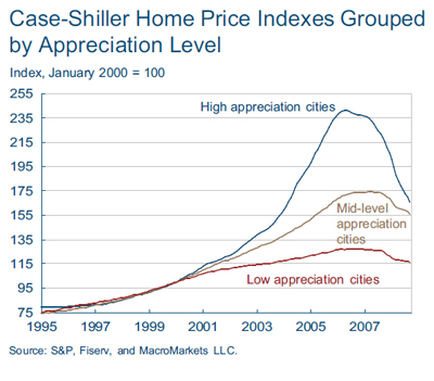
Over the relevant period, HPA actually came in a little below the -5 percent of the meltdown scenario, according to the Case-Shiller index. Reinforcing the idea that they viewed the meltdown as implausible, the analysts devoted no time to discussing the consequences of the meltdown scenario even though it is clear from tables in the paper that it would lead to widespread defaults and downgrades, even among the highly rated investment grade subprime ABS.

The authors conclude:

In the end, one has to wonder whether market participants underestimated the probability of a house price collapse or misunderstood the consequences of such a collapse. Thus, in Section 4, we describe our reading of the mountain of research reports, media commentary, and other written records left by market participants of the era. Investors were focused on issues such as small differences in prepayment speeds that, in hindsight, appear of secondary importance to the credit losses stemming from a house price
downturn. When they did consider scenarios with house price declines, market participants as a whole appear to have correctly identified the subsequent losses. However, such scenarios were labeled as “meltdowns” and ascribed very low probabilities. At the time, there was a lively debate over the future course of house prices, with disagreement over valuation metrics and even the correct index with which to measure house prices. Thus, at the start of 2005, it was genuinely possible to be convinced that nominal U.S. house prices would not fall substantially.

This is a really superb paper; so good that it will be ignored in the coming regulatory debate. The impetus to tell the story that people want to hear hasn’t changed – only the details of the story.

PrefBlog’s Assiduous Readers, however, will file this one under “Forecasting”, with a copy to “Tail Risk”.

The Parliamentary Budget Officer has released a Pre-Budget Economic and Fiscal Briefing and it makes for news that’s as bad as may be expected:

Before accounting for any new fiscal measures to be introduced in Budget 2009, this more sluggish economic outlook suggests a further deterioration in the budget balance relative to PBO’s November EFA.
o The updated economic outlook based on the PBO survey average results in a status quo budgetary deficit reaching $13 billion in 2009-10, equivalent to 0.8% of GDP.
o On a cumulative basis, status quo budget deficits amount to $46 billion over 2009-10 to 2013-14.
o PBO currently judges that the balance of risks to its fiscal outlook is tilted to the downside, reflecting the possibility of weaker-than-expected economic performance and relatively optimistic assumptions about corporate profits.
o The January survey’s low forecasts are used to illustrate potential downside economic risks and imply significantly larger deficits on a status quo basis, averaging $21 billion annually over the next five fiscal years.

…
Further, rough estimates indicate that the Government has a structural surplus of about $6 billion — though more work needs to be undertaken in this area. Thus, any permanent fiscal actions (e.g., permanent tax cuts or permanent spending increases) exceeding $6 billion annually would likely result in structural deficits, limiting the Government’s ability to manage future cost pressures due to, for example, population ageing

The total effect of the recession over the period of 2009-14, according to the average scenario (Table 2 of the report) is $45.9-billion – and this is before any special spending; the deficit arises from automatic stabilizers and revenue decreases. It will take many, many years of Spend-Every-Penny’s rosy scenarios before that money is paid back.

I have, on occasion, suggested that resource stocks make an appropriate hedge to the inflation risk embodied by a position in PerpetualDiscounts. With this in mind, it is heartening to see a Bank of Canada Discussion Paper titled Are Commodity Prices Useful Leading Indicators of Inflation?:

Commodity prices have increased dramatically and persistently over the past several years, followed by a sharp reversal in recent months. These large and persistent movements in commodity prices raise questions about their implications for global inflation. The process of globalization has motivated much debate over whether global factors have become more important in driving the inflation process. Since commodity prices respond to global demand and supply conditions, they are a potential channel through which foreign shocks could influence domestic inflation. The author assesses whether commodity prices can be used as effective leading indicators of inflation by evaluating their predictive content in seven major industrialized economies. She finds that, since the mid-1990s in those economies, commodity prices have provided significant signals for inflation. While short-term increases in commodity prices can signal inflationary pressures as early as the following quarter, the size of this link is relatively small and declines over time. The results suggest that monetary policy has generally accommodated the direct effects of short-term commodity price movements on total inflation. While indirect effects of short-term commodity price movements on core inflation have remained relatively muted, more persistent movements appear to influence inflation expectations and signal changes in both total and core inflation at horizons relevant for monetary policy. The results also suggest that commodity price movements may provide larger signals for inflation in the commodity-exporting countries examined than in the commodity-importing economies.

I will admit that the link drawn in this paper is reversed from my thesis: I am not so much concerned about what causes inflation, as I am with determining what will retain its value in the event of inflation. Still, the more links the better, say I, and I will leave for others to show a link between commodity prices and resource stock returns.

I’ve found a marvellous page on the internet, providing background material for a business course titled “MFIN 7011: Credit Risk” offered by the University of Hong Kong School of Business, taught by Dragon Yongjun Tang.

The course schedule and downloads provide some good spreadsheets for computations on the Merton Model – although the “Loffler and Posch CDS Spreadsheet” does not appear to complete, missing the function “Yearfrac()”.

Update: The “Yearfrac()” function is part of the Analysis ToolPak. In Excel, under “Tools | Add-Ins” ensure that “Analysis ToolPak – VBA” has been selected.

Neil Reynolds of the Globe had an interesting column today, Why governments can’t stop market crashes:

The formats for Prof. Smith’s market experiments vary. In one version, a number of people (traders) are given the same investment opportunity – an investment, say, that pays a 24-cent dividend every four weeks for 60 weeks. The guaranteed return is thus $3.60. In the lab setting, the times get compressed; the dividend is paid every four minutes. The traders engage in the computer-assisted buying and selling of this income stream. The process may be repeated, with variations, 15 times in a single session. Invariably, as Prof. Smith (and other economists) have repeatedly shown, traders bid each other up well beyond the actual worth of the investment. In 90 per cent of the sessions, trading ends in market crashes. Author and editor Virginia Postrel, by the way, has written a lucid and illuminating account of this research (“Pop Psychology”) in the December issue of The Atlantic magazine. Experimental economics demonstrates that people don’t normally buy and sell assets based on fundamental worth. People normally are momentum traders, trying simply to buy low and to sell high – a process that, repeated enough times, must eventually end in crashes. Laboratory research by Dutch economist Charles Noussair shows that the lab traders who make the most money are not people who determine fundamental worth; they are people who buy a lot of assets at the beginning of a trading cycle and then sell out midway through the game.

Dr. Smith’s recent paper is available through SSRN: Financial Bubbles: Excess Cash, Momentum, and Incomplete Information:

The intricate relationship between momentum and liquidity may be the chief reason for the sudden changes that occur in the markets without any apparent rationale. The overvaluation of an asset, for example, may continue as an overreaction to some new information. A small trend that is thereby established leads to buying on the part of the momentum traders. This in turn leads to a more sustained trend that continues until the available cash is too small in comparison with the asset prices. The rally then runs out of steam and appears to turn abruptly and unpredictably without any new information on fundamentals.
…
In summary, stock and other asset prices are influenced by factors beyond the market’s realistic assessment of value. The level of cash available for investment in a particular type of investment appears to be chief among them.

Note: The price evolution is shownfor six experiments, along with the straight line representing the fundamental value (which declines from $3.60 to $0.24). In the three experiments, marked by circles, in which prices soar far above the fundamental value, there is an excess of cash, the dividends are distributed at the end of each period (adding more cash) and there is a closed book so that traders do not know the entire bid–ask book. In the experiments marked by diamonds, the opposite conditions prevail, and prices remain low and there is no bubble.

I’m not sure how I can use this information, but the paper was fascinating anyway! In the meantime, the data appear to support the idea that central banks should lean against asset bubbles – the authors’ note:

In terms of world markets, the experiments suggest that the “easy money” policies of central banks lead to higher prices in financial markets. Economists often regard a nation’s stock market as a barometer of the strength of the economy, so a rising market is considered a good omen. However, from our experimental perspective, a rising market and high valuations may signify an overly relaxed monetary policy, in which assets (rather than common goods) are becoming inflated and pose a boom–bust threat.

It is generally acknowledged that central banks should not attempt to influence stock market prices, for doing so would defeat the purpose of a free market. Yet, from our perspective, the actions of central banks have a profound influence on the price levels of markets. The expansion of price/earnings ratios in U.S. stocks during the mid-1990s may have been enhanced by the Federal Reserve’s easing of monetary policy in response to the savings and loan crisis. Similarly, the Fed’s easing of interest rates during the fall of 1998, this time in response to the insolvency of Long Term Capital Management, and the precautionary increase in liquidity in anticipation of a Year 2000 problem, occurred during a time of economic expansion and may have contributed to the bubble of 1999.

A query regarding Graham’s position on preferred stock came to my attention, so I looked it up:

Certain general observations should be made here on the subject of preferred stocks. Really good preferred stocks can and do exist, but they are good in spite of their investment form, which is an inherently bad one. The typical preferred shareholder is dependent for his safety on the ability and desire of the company to pay dividends on its common stock. Once the common dividends are omitted, or even in danger, his own position becomes precarious, for the directors are under no obligation to continue paying him unless they also pay on the common. On the other hand, the typical preferred stock carries no share in the company’s profits beyond the fixed dividend rate. Thus the preferred holder lacks both the legal claim of the bondholder (or creditor) and the profit possibilities of a common shareholder (or partner).

These weaknesses in the legal position of preferred stocks tend to come to the fore recurrently in periods of depression. Only a small percentage of all preferred issues are so strongly entrenched as to maintain an unquestioned investment status through all vicissitudes.

Experience teaches that the time to buy preferred stocks is when their price is unduly depressed by temporary adversity. (At such times they may be well suited to the aggressive investor but too unconventional for the defensive investor.)

In other words, they should be bought on a bargain basis or not at all.
…
Another peculiarity in the general position of preferred stocks deserves mention. They have a much better tax status for corporation buyers than for individual investors. Corporations pay income tax on only 15% of the income they receive in dividends, but on the full amount of their ordinary interest income. Since the 1972 corporate rate is 48%, this means that $100 received as preferred-stock dividends is taxed only $7.20, whereas $100 received as bond interest is taxed $48. On the other hand, individual investors pay exactly the same tax on preferred-stock investments as on bond interest, except for a recent minor exemption. Thus, in strict logic, all investment-grade preferred stocks should be bought by corporations, just as all tax-exempt bonds should be bought by investors who pay income tax.

In the last paragraph, Mr. Graham recognizes that tax differences are important – very important! Using his figures the equivalency ratio within a corporation is a stunning 1.9x – in other words, it took $1.90 in interest to provide the same after tax income as $1.00 in dividends. For an individual, the equivalency ratio was 1:1.

It seems quite clear to me that under these conditions there will be very little left on the table for individual investors – Mr. Graham’s target audience – after corporations have picked through the offerings.

Other than this, the passage is sorely lacking in numeric analysis and opinion based on specific fact. Mr. Graham acknowledges that there is some price – some yield – at which a preferred share becomes superior to a given bond, but does not provide any analytical framework that will allow an interested reader to determine how that price – that yield – might be determined.

The market has changed dramatically since the early ’70’s. Besides the taxation differences between US-then and Canada-now already noted, there are regulatory elements in play that make preferred shares an attractive way to raise capital for banks and some utilities.

However, my main objection to the passage is that it is too rigidly doctrinaire. The world as presented is black and white, with safety on one side and profit on the other. In fact, the real world contains many shades of grey, which are ignored.

The revised edition cited contains further commentary by Jason Zweig:

Preferred shares are a worst-of-both-worlds investment. They are less secure than bonds, since they have only a secondary claim on a company’s assets if it goes bankrupt. And they offer less profit potential than common stocks do, since companies typically “call” (or forcibly buy back) their preferred shares when interest rates drop or their credit rating improves. Unlike the interest payments on most of its bonds, an issuing company cannot deduct preferred dividend payments from its corporate tax bill. Ask yourself: If this company is healthy enough to deserve my investment, why is it paying a fat dividend on its preferred stock instead of issuing bonds and getting a tax break? The likely answer is that the company is not healthy, the market for its bonds is glutted, and you should approach its preferred shares as you would approach an unrefrigerated dead fish.

For all his colourful language, Mr. Zweig shows lamentable ignorance of bank regulation; this is perhaps partly due to his exclusive focus on the American market, in which dividends are taxable to an investor at the same rate as interest; hence the market is much less vibrant in the US than in Canada.

I will certainly agree with Mr. Zweig’s emphasis on the undesirability of call features – but a call is simply another element of investment risk, to be calculated and incorporated when determining the value of an asset.

I will note that according to his biography, Mr. Zweig is a journalist, not an analyst or portfolio manager. It is therefore not possible to gauge the value of his opinions by reference to his results.

The Bank of England has released Working Paper #358, “Understanding the real rate conundrum: an application of no-arbitrage finance models to the UK real yield curve”, by Michael Joyce, Iryna Kaminska and Peter Lildholdt, with the abstract:

Long-horizon interest rates in the major international bond markets fell sharply during 2004 and 2005, at the same time as US policy rates were rising; a phenomenon famously described as a ‘conundrum’ by Alan Greenspan the Federal Reserve Chairman. But it was arguably the decline in international long real rates over this period which was more unusual and, by the end of 2007, long real rates in the United Kingdom remained at recent historical lows. In this paper, we try to shed light on the recent behaviour of long real rates, by estimating several empirical models of the term structure of real interest rates, derived from UK index-linked bonds. We adopt a standard ‘finance’ approach to modelling the real term structure, using an essentially affine framework. While being empirically tractable, these models impose the important theoretical restriction of no arbitrage, which enables us to decompose forward real rates into expectations of future short (ie risk-free) real rates and forward real term premia. One general finding that emerges across all the models estimated is that time-varying term premia appear to be extremely important in explaining movements in long real forward rates. Although there is some evidence that long-horizon expected short real rates declined over the conundrum period, our results suggest lower term premia played the dominant role in accounting for the fall in long real rates. This evidence could be consistent with the so-called ‘search for yield’ and excess liquidity explanations for the conundrum, but it might also partly reflect strong demand for index-linked bonds by institutional investors and foreign central banks.

From the discussion:

One clear finding of our results across all the models we estimate is the importance of movements in estimated real term premia in explaining movements in real rates. This is contrary to what appears to be the conventional wisdom that real term premia are small and negligible. Indeed, many papers simply ignore the presence of real term premia altogether (for a recent example, see Ang, Bekaert and Wei (2007)).
…
Negative term premia are of course quite consistent with finance theory and may indicate that for some investors long-maturity index-linked bonds are seen as providing a form of ‘insurance’. However, the emergence of negative term premia in the late 1990s seems likely to have reflected the impact of various accounting and regulatory changes that have caused pension funds to match their assets more closely to their liabilities by switching into long-maturity conventional and index-linked bonds (see McGrath and Windle (2006)). Indeed, the timing of the move to negative term premia suggested by the model decompositions seems to broadly match the introduction of the MFR in 1997, which market commentary suggests had a significant impact on UK pension fund asset allocation.

Footnote: More recently, the Pensions Act 2004, which became effective in December 2005, introduced a new Pensions Regulator with powers to require pension fund trustees and sponsors to address issues of underfunding. Another factor that may also have influenced pension fund behaviour has been the ‘FRS 17’ accounting standard, which became effective from the start of 2005, and has meant that pension scheme deficits/surpluses need to be measured at market value and included on company balance sheets. Both these factors are thought to have increased pension fund demand for longer-duration nominal and real gilts, as assets which provide a better match for their liabilities. See discussion in the ‘Markets and Operations’ article of the Bank of England Quarterly Bulletin, Spring 2006.

With conclusions:

Another important finding, common to all the estimated model specifications, is that our term premia estimates appear to have been negative over much of the sample period since the late 1990s. We have argued that this is likely to reflect the impact of various accounting and regulatory changes in the United Kingdom that have encouraged pension funds to match their assets more closely to their liabilities, by switching into long-maturity conventional and index-linked bonds. The importance of this Category 3 explanation for the behaviour of term premia after the 1990s needs to be borne in mind when interpreting more recent downward moves in term premia.
…
In terms of understanding the fall in long rates over the conundrum period during 2004 and 2005, all the estimated models suggest that falls in UK long real rates have to a significant degree reflected reductions in real term premia, though the extent to which this is true varies with the precise model specification used. The importance of the reduction in term premia might indicate the influence of changing institutional investor behaviour, but the fact that the decline in long rates was a global phenomenon suggests to us that this is unlikely to have been the primary cause. This leads us to the conclusion that excess liquidity and search for yield were more important in explaining the compression of real term premia. But since our models also suggest that there is some evidence that perceptions of the neutral rate of interest may have fallen, we cannot rule out the possibility that changes in the balance of investment and saving may also have had an impact. In terms of the recent conjuncture, all our model specifications would suggest that there is a risk real rates may rise in the future, since in all of the models forward premia or expected future short rates are below their long-run expected levels.

Chart 6: Decomposition of the ten-year real forward rate from the survey model:

The Cleveland Fed has released the December issue of Economic Trends, with articles:

• October Price Statistics
• The Yield Curve, November 2008
• Japan’s Quantitative Easing Policy
• Industrial Production, Commodity Prices, and the Baltic Dry Index
• GDP: Third Quarter Preliminary Estimate
• The Employment Situation, October 2008
• Metro-Area Differences in Home Price Indexes
• Fourth District Employment Conditions, October 2008
• Fourth District Community Banks

One table and one chart are of particular interest:

Deflation is always a possibility, but for now it looks like a simple unwind of the commodity boom.

Houses, ditto.

Cities like Miami, Los Angeles, San Diego, and Washington, D.C. all saw tremendous growth in home prices during the boom and have all subsequently seen massive declines in values. On the other hand, cities like Denver and Charlotte saw little to no unusual home price appreciation during the boom and have seen home prices decline only modestly during the bust.

Bank Sub-Debt has been in the news lately, with Deutsche Bank’s refusal to execute a pretend-maturity, and I have dug up another theoretical paper: What does the Yield on Subordinated Bank Debt Measure, by Urs W. Birchler (Swiss National Bank) & Diana Hancock (Federal Reserve):

We provide evidence that the yield spread on banks’ subordinated debt is not a good measure of bank risk. First, we use a model with heterogeneous investors in which subordinated debt is primarily held by investors with superior knowledge (i.e., the“informed investor hypothesis”). Subordinated debt, by definition, coexists with non-subordinated, or “senior,” debt. The yield spread on subordinated debt thus must not only compensate investors for expected risk (i.e., to satisfy their participation constraint), but also offer an “incentive premium” above a “fair” return to induce informed investors to prefer it to senior debt (i.e., to satisfy an incentive constraint). Second, we test the model using data we collected on the timing and pricing of public debt issues made by large U.S. banking organizations in the 1986-1999 period. Findings with respect to issuance decisions lend strong support for the informed investor hypothesis. But rival explanations for the use of subordinated debt, such as differences in investor risk aversionor such as the signaling of earnings prospects by the bank, are rejected.A sample selection model on observed issuance spreads provides evidence for the existence of the postulated subordinated incentive premium. In line with predictions from the model, the influence of sophisticated investors’ information on the subordinated yield spread became weaker after the introduction of prompt corrective actions and depositor preference regulatory reforms, while the influence of public risk perception grew stronger. Finally, our model explains some results from the empirical literature on subordinated debt spreads and from market interviews — such as limited spread sensitivity to bank specific-risk or of the “ballooning” of spreads in bad times.

The conclusions are consistent with those of other researchers.

There’s a good line in the discussion:

These results are consistent with the “informed investor hypothesis” that claims that banking organizations would issue debt of different priority status to separate investors with different, yet unobservable, beliefs on the probability of bank failure.

I claim that a good definition of an “informed investor”, suitable for ex ante assignment of investors into different groups is: “one who knows that there is a difference”. The authors would not, I think, disagree too violently with this definition:

Paradoxically, the quality of the subordinated debt spread to measure banking organizations’ risks as they are perceived by most sophisticated investors has deteriorated after the introduction of FDICIA or, more precisely, of depositor preference rules. With depositor preference rules, the risk characteristics of senior debt have become more similar to those of subordinated debt; at the same time, the subordinated debt spread has become (even) more dependent on factors influencing the senior spread.

The deterioration of the risk measurement quality of the subordinated spread after the introduction of depositor preference, however, is likely to understate the longer term virtues of the reform. Once senior debtors realize that their claims are subordinated to depositors, senior spreads may well more fully reflect specialist information. Therefore, we expect that senior debt will be held by more sophisticated investors in the future.

Assiduous Readers will remember that in my essay on Fixed-Reset Analysis I pointed out a very low spread between deposit notes and sub-debt in February 2007.